4  Embeddings — Numbers to Meaning

We have token IDs: [10, 3, 4, 8]. They are integers. The model cannot do useful math on raw integers — adding 10 + 3 gives 13, which means nothing. To do useful math, each integer needs to become a vector — a list of numbers that encodes the token’s meaning geometrically.

The mechanism is called the embedding matrix, and it is the model’s first learned representation.

4.1 The Idea

To give each token a meaning the model can actually compute with, we replace its ID with a list of hundreds of decimal numbers — a vector. Think of it like this: the model keeps a big table, one row per word in the vocabulary. When it sees token 42, it pulls out row 42 and uses those numbers as the token’s representation going forward.

The key property that makes this useful is that the table is learned. After training on billions of words, tokens with similar meanings end up with similar rows. “Cat” and “kitten” cluster together. “Run” and “sprint” are nearby. “Cat” and “justice” are far apart. The model discovers these relationships entirely from how words appear together in text — no human labels required.

This learned table is the embedding matrix, and the step that converts a sequence of IDs into a sequence of vectors is called embedding.

4.2 Why Learned Vectors?

The values in the embedding matrix are not hand-crafted. They are initialized randomly and then learned via gradient descent during training, just like any other model parameter.

Math Minute — Gradient Descent

Gradient descent is the basic training rule: measure the model’s error, compute which direction would increase that error, then nudge each parameter a small step in the opposite direction. Repeated millions or billions of times, these tiny updates turn random numbers into useful weights. For embeddings, that means each token’s row moves toward values that help the model predict text better.

The training objective is next-token prediction: given \(t_1, t_2, \ldots, t_n\), predict \(t_{n+1}\). Because the model must do this well across billions of examples, it is forced to arrange embeddings such that tokens that appear in similar contexts land near each other in the embedding space.

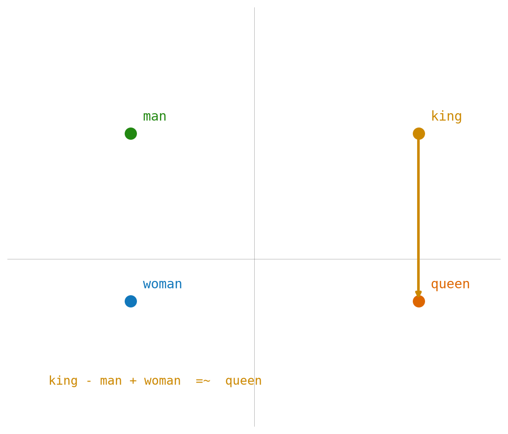
This produces the famous arithmetic property:

\[ \mathrm{embedding}(\mathrm{king}) - \mathrm{embedding}(\mathrm{man}) + \mathrm{embedding}(\mathrm{woman}) \approx \mathrm{embedding}(\mathrm{queen}) \]

No one programmed this. It is a geometric consequence of how the vectors were shaped by the training signal.

4.3 The Math

The embedding matrix \(E \in \mathbb{R}^{|V| \times d}\) holds one learned row per token — \(|V|\) tokens wide, \(d_{\text{model}}\) dimensions deep. To embed token \(i \in \{0, \ldots, |V|-1\}\), we pull out its row:

\[ e_i = E_{i,\cdot} \in \mathbb{R}^d \]

For a sequence of \(T\) tokens \([i_1, \ldots, i_T]\), we collect the corresponding rows into a matrix:

\[ X = E[[i_1,\ldots,i_T], :] \in \mathbb{R}^{T \times d} \]

Row indexing, no arithmetic. We can also write the same lookup as a matrix multiplication using a one-hot vector:

\[ e_i = o_i^{\top} \cdot E, \quad \text{where } o_i \in \{0,1\}^{|V|},\quad (o_i)_j = \begin{cases} 1 & j = i \\ 0 & j \neq i \end{cases} \]

The one-hot form shows up in theoretical derivations, but implementations skip it and index directly — it is much faster.

Math Minute — One-Hot Vector

A one-hot vector has exactly one entry equal to \(1\) and all others \(0\). Token ID \(2\) in a vocabulary of size 5 becomes:

\[ o_2 = [0, 0, 1, 0, 0] \]

Multiplying \(o_2^{\top}\) by \(E\) selects row 2 — the same result as \(E_{2,\cdot}\).

4.4 The Matrix: Worked Example

Take tiny numbers: \(|V| = 5\), \(d = 4\).

Embedding matrix \(E\) (\(5\times 4\)):

       col0   col1   col2   col3
tok 0: [ 0.10  -0.20   0.30  -0.40 ]
tok 1: [ 0.50   0.60  -0.70   0.80 ]
tok 2: [-0.90   0.10   0.20  -0.30 ]
tok 3: [ 0.40  -0.50   0.60  -0.70 ]
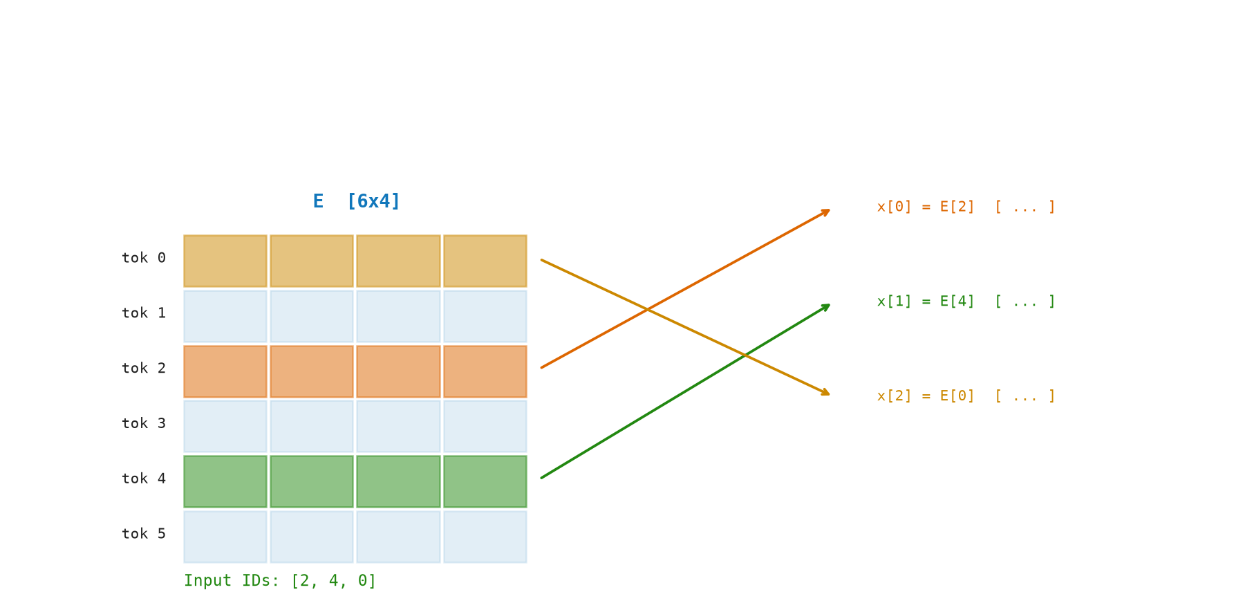
tok 4: [-0.10   0.80  -0.40   0.50 ]

Input token sequence: "low lower" → token IDs [2, 3, 0] (hypothetical).

Embedding lookup:

X = E[[2, 3, 0], :]

X[0] = E[2] = [-0.90,  0.10,  0.20, -0.30]   ← "low"
X[1] = E[3] = [ 0.40, -0.50,  0.60, -0.70]   ← "low" (part of "lower")
X[2] = E[0] = [ 0.10, -0.20,  0.30, -0.40]   ← "er"

Result X: shape [3 × 4]

This \([3 \times 4]\) matrix is what flows into the next stage.

Figure Figure 4.1 shows token IDs selecting row vectors from the embedding matrix.

Figure 4.1: Token IDs mapped to embedding rows

Semantic similarity in vector space:

If we compute the dot product of two token embeddings, we get a scalar measuring how aligned they are:

dot(E[0], E[2]) = (0.10)(−0.90) + (−0.20)(0.10) + (0.30)(0.20) + (−0.40)(−0.30)
              = −0.09 − 0.02 + 0.06 + 0.12
              = 0.07   (slightly positive → slight similarity)

After training, semantically related tokens will have much higher dot products.

4.5 The Code: Embedding in Python

Chapter 3 already showed how text becomes token IDs. Here we start from those IDs and look up vectors.

def make_matrix(rows: int, cols: int, fill: float = 0.0) -> Matrix:
    return [[fill for _ in range(cols)] for _ in range(rows)]


def shape(matrix: Matrix) -> tuple[int, int]:
    return len(matrix), len(matrix[0]) if matrix else 0

This helper creates a rows-by-cols grid of numbers. The embedding matrix uses the same matrix abstraction introduced earlier, so chapter 4 does not need a new data structure.

def random_matrix(
    rows: int,
    cols: int,
    rng: random.Random,
    scale: float | None = None,
) -> Matrix:
    scale = math.sqrt(2.0 / (rows + cols)) if scale is None else scale
    return [[rng.uniform(-scale, scale) for _ in range(cols)] for _ in range(rows)]

random_matrix fills that grid with small random values. With the default Xavier scale, the random values are sized by \(\sqrt{2/(fan_{in}+fan_{out})}\) so activations are less likely to explode or vanish.

def embed_token(embedding: Matrix, token_id: int) -> Vector:
    return list(embedding[token_id])

The embedding of token \(i\) is row \(i\) of the matrix. This is a table lookup, not a calculation over the token ID itself.

def embed_sequence(embedding: Matrix, token_ids: Sequence[int]) -> Matrix:
    return [embed_token(embedding, token_id) for token_id in token_ids]

A sequence of \(T\) token IDs becomes \(T\) row lookups stacked into a \([T \times d]\) matrix. The vector helpers used to compare rows are the same ones from Chapter 2.

Demo. Run with python3 src/python/chapter_demos.py:

def chapter_04(seed: int = 4) -> dict[str, object]:
    rng = random.Random(seed)
    embedding = random_matrix(100, 8, rng)
    x = embed_sequence(embedding, [1, 2, 3])
    return {
        "sequence_shape": (len(x), len(x[0])),
        "dot": dot(embedding[1], embedding[2]),
        "cosine": cosine_similarity(embedding[1], embedding[2]),
    }

The demo starts with token IDs, creates an embedding table, and returns the embedded sequence shape. It also compares two embedding rows with dot product and cosine similarity, reusing the chapter 2 helpers instead of repeating them here.

Figure Figure 4.2 shows how each token ID indexes into one row of the embedding weight matrix.

Figure 4.2: Embedding matrix lookup

Figure Figure 4.3 shows how semantic relationships can appear as vector directions in embedding space.

Figure 4.3: Semantic arithmetic in embedding space

4.6 Key Takeaways

• An embedding matrix \(E \in \mathbb{R}^{|V| \times d}\) maps token IDs to dense vectors.
• The embedding of token i is row i of E — a single lookup, no computation.
• For a sequence of T tokens, we get a \([T \times d]\) matrix X.
• The vectors are learned: training nudges similar tokens closer together.
• Semantic arithmetic (\(\text{king} - \text{man} + \text{woman} \approx \text{queen}\)) emerges from the training objective.

What’s next? We have a matrix X of shape \([T \times d]\). Each row knows what the token is, but nothing about where it sits in the sequence. Swapping two tokens would produce the same rows in a different order, which the model would treat identically. We need to inject position information — that is Chapter 5.