11 Vocabulary Projection — From Vectors to Words
After N transformer blocks, we have a matrix \(X_{\text{final}} \in \mathbb{R}^{T\times d}\). The final row, X_final[T-1], is a rich contextualized representation of the last token. The last step is to project this vector into a probability distribution over the vocabulary: which token is most likely to come next?
This projection is called the language model head, or unembedding layer.
11.1 The Idea
After all the attention and feed-forward layers, we have a vector representing the last token — a list of hundreds of numbers that encodes everything the model knows about what has been said so far. But the user needs a word, not a list of numbers.
The final step converts that vector into a probability over the entire vocabulary: for each of the 50,000-odd words the model knows, what is the chance it is the right next word? The word with the highest probability (or a word sampled from the distribution) becomes the model’s output.
How does a vector become a probability distribution? The model compares the vector against every word in the vocabulary and assigns a score to each one. High score means “this word fits the context well.” Low score means it does not. Then those scores are squeezed into the range 0–1 and made to sum to 1, giving a proper probability.
This step is the mirror image of Chapter 4: embedding turned an integer (a word ID) into a vector; unembedding turns a vector back into a distribution over integers. Many implementations reuse the same table for both directions: the same weights that encode “cat → vector” are transposed to decode “vector → how much does this look like cat?”
11.2 The Math
Given the final hidden state \(h_t = X_{\text{final}}[T-1] \in \mathbb{R}^d\):
Step 1 — Final Layer Norm:
\[ \tilde{h}_t = \operatorname{LayerNorm}(h_t) \in \mathbb{R}^d \]
Step 2 — Vocabulary Projection:
\[ \text{logits} = \tilde{h}_t W_u \in \mathbb{R}^{|V|} \]
With weight tying: \(W_u = E^{\top}\), so:
\[ \text{logits}[i] = \tilde{h}_t \cdot E_i \]
The logit for token i is the dot product of the model’s “prediction vector” with token i’s embedding. Tokens whose embeddings align with the prediction vector get high logits.
Step 3 — Softmax → Probabilities:
\[ P(\text{next} = i \mid \text{context}) = \operatorname{softmax}(\text{logits})[i] = \frac{\exp(\text{logits}[i])}{\sum_j \exp(\text{logits}[j])} \]
Math Minute — Temperature
We can control the “sharpness” of the distribution with a temperature parameter \(T_{\text{temp}}\):
\[ P(i) = \operatorname{softmax}(\text{logits} / T_{\text{temp}})[i] \]
- \(T_{\text{temp}} \to 0\): argmax — always pick the highest-probability token (greedy)
- \(T_{\text{temp}} = 1\): standard softmax
- \(T_{\text{temp}} > 1\): flattens the distribution — more randomness/creativity
Temperature is not a model parameter — it’s a sampling hyperparameter set at inference time.
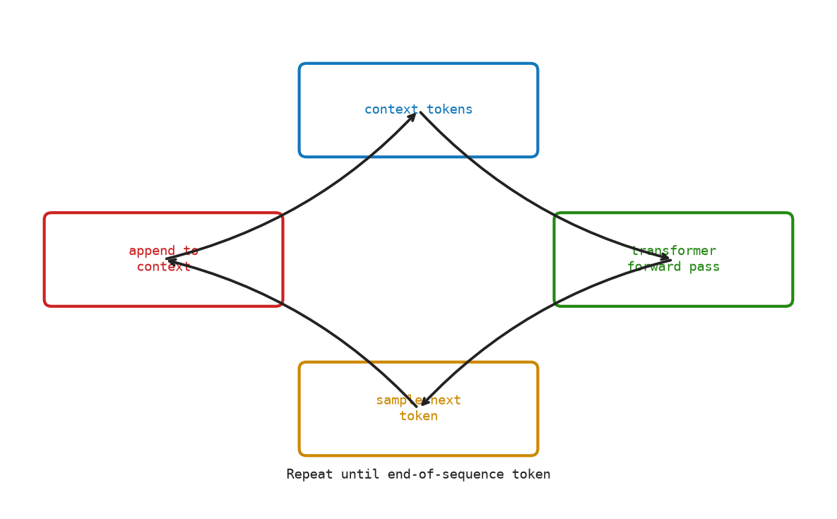
11.3 The Generation Loop
Training and inference use the same forward pass differently.
Training: Given a sequence \([t_1, t_2, \ldots, t_n]\), the model predicts all next tokens simultaneously (thanks to causal masking): \(P(t_2|t_1), P(t_3|t_1,t_2), \ldots\). The loss is cross-entropy averaged over all positions.
Inference (generation):
- Start with prompt tokens \([t_1, \ldots, t_n]\)
- Forward pass → logits for position \(n\)
- Sample or \(\mathrm{argmax}\) → \(t_{n+1}\)
- Append \(t_{n+1}\) to the sequence
- Forward pass → logits for position \(n+1\)
- Repeat until stop token or max length
This is called autoregressive generation: each new token is fed back in as input to generate the next.
11.4 The Matrix: Worked Example
Let |V| = 5, d = 4. Final hidden state:
h = [0.3, -0.1, 0.8, 0.2]Unembedding matrix \(W_u = E^{\top}\) (columns = token embeddings):
logits[0] = h · E[0] = (0.3)(0.10) + (-0.1)(−0.20) + (0.8)(0.30) + (0.2)(−0.40)
          = 0.030 + 0.020 + 0.240 − 0.080 = 0.210

logits[1] = h · E[1] = 0.150 − 0.060 − 0.560 + 0.160 = −0.310
logits[2] = h · E[2] = −0.270 − 0.010 + 0.160 − 0.060 = −0.180
logits[3] = h · E[3] = 0.120 + 0.050 + 0.480 − 0.140 = 0.510
logits[4] = h · E[4] = −0.030 − 0.080 − 0.320 + 0.100 = −0.330

logits = [0.210, -0.310, -0.180, 0.510, -0.330]
Softmax:
exp(logits) = [1.233, 0.733, 0.835, 1.665, 0.719]
sum         = 5.185

P = [0.238, 0.141, 0.161, 0.321, 0.139]
Token 3 has the highest probability (32.1%). That is the top-ranked token for this context.
Figure Figure 11.1 shows the vocabulary projection converting a hidden state into logits over the vocabulary.
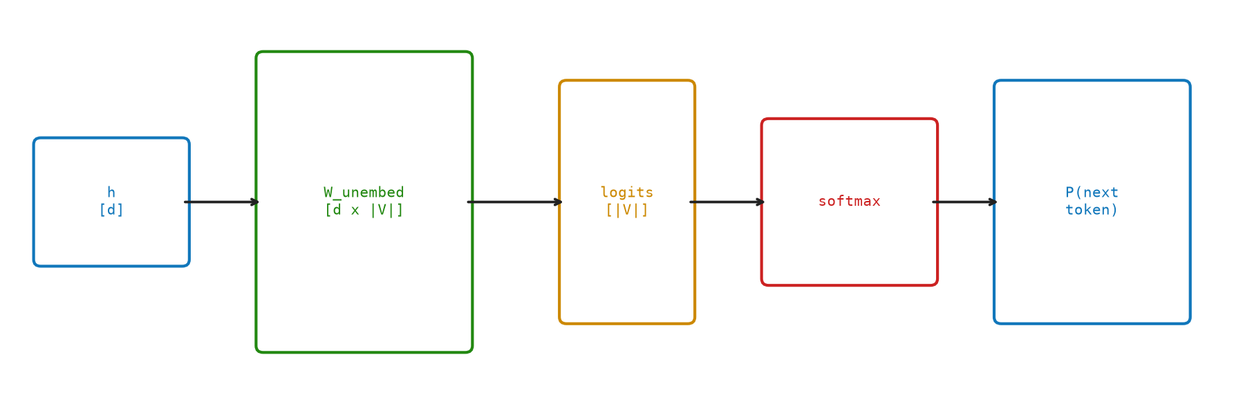
Figure Figure 11.2 shows autoregressive generation, where each predicted token is appended and fed back into the model.
11.5 The Code: Full microGPT Forward Pass in Python
@dataclass(frozen=True)
class GPTConfig:
    vocab_size: int
    d_model: int
    num_heads: int
    num_layers: int
    max_seq_len: int
Configuration is data. GPTConfig stores the model’s five hyperparameters in one immutable object.
@dataclass
class GPTParams:
    wte: Matrix
    wpe: Matrix
    blocks: list[TransformerBlock]
    ln_f: LayerNorm


def make_gpt_params(config: GPTConfig, rng: random.Random) -> GPTParams:
    return GPTParams(
        wte=random_matrix(config.vocab_size, config.d_model, rng),
        wpe=random_matrix(config.max_seq_len, config.d_model, rng),
        blocks=[
            make_transformer_block(config.d_model, config.num_heads, rng)
            for _ in range(config.num_layers)
        ],
        ln_f=make_layer_norm(config.d_model),
    )
make_gpt_params allocates all learnable weights. wte is the token embedding matrix \([|V| \times d]\); wpe is the position embedding matrix. Weight tying means the unembedding step will reuse wte transposed, so no separate parameter is stored.
def gpt_forward(token_ids: Sequence[int], params: GPTParams, config: GPTConfig) -> Vector:
    if len(token_ids) > config.max_seq_len:
        raise ValueError("token_ids exceeds max_seq_len")

    token_embeddings = embed_sequence(params.wte, token_ids)
    position_embeddings = embed_sequence(params.wpe, range(len(token_ids)))
    x = matrix_add(token_embeddings, position_embeddings)
    x = forward_stack(x, params.blocks)
    h = layer_norm_vector(x[-1], params.ln_f)
    return [dot(h, token_vector) for token_vector in params.wte]
gpt_forward is the full pipeline: embed token IDs, add position embeddings, pass through \(N\) transformer blocks, apply the final layer norm to the last token’s vector, then compute dot products with every row of wte.
def temperature_scale(logits: Sequence[float], temperature: float) -> list[float]:
    return [value / temperature for value in logits]


def top_k_filter(logits: Sequence[float], k: int) -> list[float]:
    keep = {index for index, _value in sorted(enumerate(logits), key=lambda item: item[1], reverse=True)[:k]}
    return [value if index in keep else -1.0e9 for index, value in enumerate(logits)]


def sample_token(probabilities: Sequence[float], rng: random.Random) -> int:
    threshold = rng.random()
    cumulative = 0.0
    for index, probability in enumerate(probabilities):
        cumulative += probability
        if threshold <= cumulative:
            return index
    return len(probabilities) - 1


def generate(
    params: GPTParams,
    config: GPTConfig,
    start_ids: Sequence[int],
    max_new_tokens: int,
    temperature: float,
    top_k: int,
    rng: random.Random,
) -> list[int]:
    tokens = list(start_ids)
    generated = []
    for _ in range(max_new_tokens):
        logits = gpt_forward(tokens, params, config)
        probabilities = softmax(top_k_filter(temperature_scale(logits, temperature), top_k))
        next_token = sample_token(probabilities, rng)
        tokens.append(next_token)
        generated.append(next_token)
    return generated
generate is the autoregressive loop. It repeatedly runs the model, scales and filters the logits, samples one next token, appends it to the context, and continues.
Run with python3 src/python/chapter_demos.py.
11.6 Weight Tying in Detail
Why does weight tying work so well?
- The embedding
E[i]is learned to represent tokenisuch that tokens that appear in similar contexts have similar embeddings. - The unembedding \(\text{logits}[i] = h \cdot E[i]\) measures the alignment between the model’s prediction vector
hand tokeni’s embedding. - If
his pointing in the direction of “tokens that follow this context,” andE[i]represents tokeni’s meaning, then tokens that are semantically appropriate will naturally score higher.
Weight tying forces the model to use a single geometric space for both “what a token means” and “how to predict a token,” a constraint that also regularizes learning.
11.7 Key Takeaways
- The unembedding projects the final hidden state to logits: \(\text{logits} = h W_u \in \mathbb{R}^{|V|}\).
- Weight tying (\(W_u = E^{\top}\)) reuses the embedding matrix and reduces parameters.
- Softmax converts logits to a probability distribution.
- Temperature controls sampling sharpness; top-K restricts the candidate set.
- Autoregressive generation: sample one token at a time, feeding each back as input.
11.8 The Complete Picture
You have now seen every piece:
Input text
   ↓ tokenizer
Token IDs: [3, 7, 12, 5, …]
   ↓ embedding matrix E
Token embeddings: [T × d]
   ↓ + positional encoding
X̃ = X + PE: [T × d]
   ↓ transformer block × N
   │   LayerNorm
   │   Multi-Head Attention (Q, K, V projections + causal mask + softmax + weighted sum)
   │   Residual
   │   LayerNorm
   │   Feed-Forward Network (expand → GELU → contract)
   │   Residual
   ↓
X_final: [T × d]
   ↓ final LayerNorm + unembedding
Logits: [|V|]
   ↓ softmax (+ temperature + top-K)
P(next token): [|V|]  →  sample  →  next token ID
Every box in that diagram corresponds to one chapter of this book.